In this article, we are going to explore an application of an autonomous driving vehicle using reinforcement learning. First, we introduce the basic theory behind the control system of an autonomous ground vehicle (AGV). Then we simulate some AGV examples using an open source library denominated Python Robotics. Finally, we present how we can optimize the AGV speed using a traditional reinforcement learning method. In this regard, the following contributions can be highlighted:
- Introducing some basic theory of autonomous vehicle model;
- Applying Python Robotics open source library to simulate AGVs.
- Presenting a reinforcement learning solution to optimize the AGV speed.
- Autonomous Ground Vehicle (AGV)
Here we describe a simplified kinematic model that characterize the vehicle movement over a set of differential equation. More detailed and deeper explanation of many state-of-the-art vehicle models can be found in [1].
Consider the vehicle of Fig. 1, where its rear wheel position is located at (x,y), with distance L from the front wheel and heading angle θ describing the direction that the vehicle is facing. In fact, we can define the triple (x(t), y(t), θ(t)) to describe the vehicle current state at a certain time t.
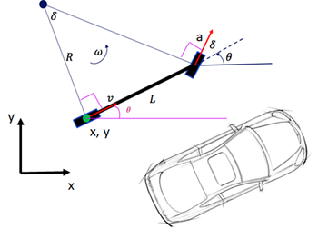
Controlling the vehicle direction and its speed means that we want to update the vehicle’s state to a new position, such that we have (x(t+1), y(t+1), θ(t+1)) converging toward the desired location. Hence, we can define a steering angle δ and acceleration a, as presented in Fig. 1, to be applied at the current vehicle’s state, where the positions of the AGV are updated according to the following differential equations:
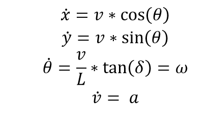
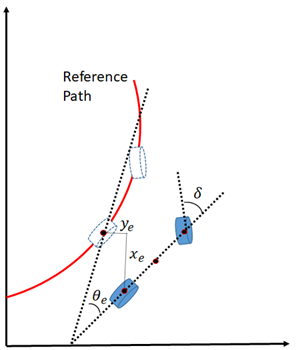
So, supposing we previously defined a reference path in which the vehicle must follow, the control process is based on calculating the error of the AGV current state at time t: and fixing it using (δ, a). This is represented in Fig. 2.
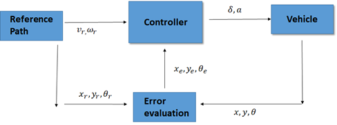
Finding the best way to calculate (δ, a) has been for many years the subject of study of many control engineers and, as you can expect, there are different solutions for this control problem. We recommend the paper in [1] as a very nice survey of various control strategies. The Fig. 3 provides a summary of the general control process. Basically, the AGV reports its current state (x,y,θ), such that it’s then used for calculating the error to the reference trajectory (x_r,y_r,θ_r), thus generating (x_e,y_e,θ_e). This error serves as input to the controller, which also takes the reference trajectory linear speed (v_r) and angular speed (ω_r) to provide the control command (δ,a) that will further adjust the AGV position.
2. Simulating an AGV using Python Robotics Library
Here we are going to explore the library developed by the authors in [2] for simulating an autonomous vehicle trajectory following. The code is provided in https://github.com/AtsushiSakai/PythonRobotics
There you can find other examples rather than autonomous vehicle use cases, such aerial navigation and robot arms.
In our AGV example, let’s analyze the Stanley controller, the winner of the DARPA’s Grand Challenge in 2005, developed by the researchers of Stanford University. The Stanley controller’s code can be found in: /PythonRobotics/PathTracking/stanley_controller/stanley_controller.py
We’d like to emphasize basically three main parts of this code, the first one at the main() function:
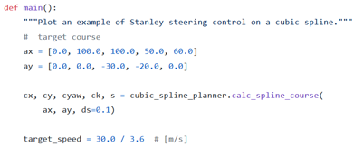
These first lines describes the Reference path the AGV must follow. The variables cx and cy represents the positions x and y the AGV must to follow throughout the path. The target_speed variable defines the desired speed you want the AGV to achieve.
After that, we have the following:

This is the main loop of the algorithm. It means that the AGV keeps updating its positions until 1) The simulation time surpass a certain defined value (it means the AGV couldn’t achieve the final destination the time given) and 2) The AGV achieved its last waypoint (it means the final goal was reached).
You can also note that there are two main variables being calculated at each time step: ai and di. Both represents the control signal for the acceleration and the steering angle. The acceleration is obtained by a PID controller and the Steering angle using the Stanley’s control law. The theory of Stanley’s control law can be found in more details at [3].
It’s also interesting to highlight that after the control signal is generated, the AGV applies its information for state update: state.update(ai, di). At the update method, we can check:
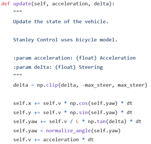
Note how the positions x,y, theta and v are updated giving the control command for a time step dt. Let’s now run the algorithm to check what it returns:
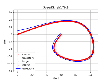
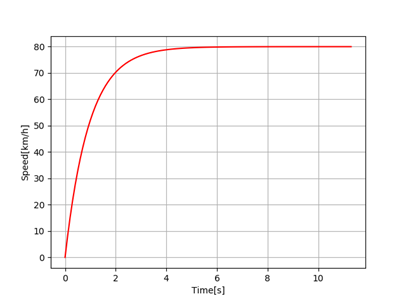
So, two plots were generated. The first one showing the AGV positions through time, where it tries to follow the reference trajectory. The second plot show the speed variation also through time, showing the AGV increasing its speed until reaching the desired speed we selected (in this case, 80 km/h) with a timestep dt = 0.1 s.
As you can note, in this scenario, everything works fine, however, regardless the curve of the path, the AGV still tries to do it with the desired speed of 80 km/k. A direct consequence of this reckless behavior is that at the end of the trajectory, which contains a sharper curve, the difference between the desired trajectory and the current trajectory increased substantially. In other words, the AGV got out of the road. To check further this performance difference, let’s make the same simulation for 40 km/h target speed case:
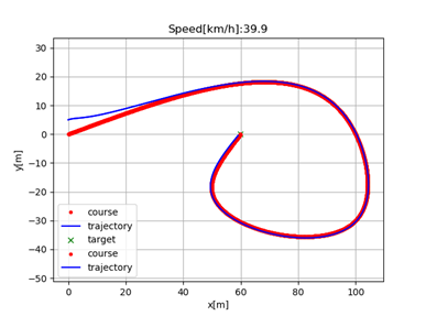
As you can visually note, the error between the AGV path and the reference is much lower.
There’s actually a metric very used in current literature to define this quantity represented by “how much error exists between the AGV current trajectory and reference trajectory”, named cross-track error (XTE):
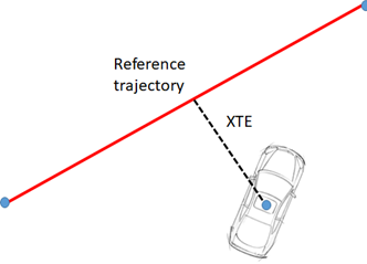
The cross track error is defined by the minimum distance of the vehicle current position to the reference trajectory. This metric is actually strongly used for many applications of navigational dynamics, such as vehicles, airplanes and ships.
3. Reinforcement Learning for Controlling the Speed
In previous section, we noted that higher speeds cause high cross-track error, especially if there is sharp curves throughout the path. However, the target speed is a fixed variable. The controller is not aware of the path circumstances, it just provides control information to the AGV achieve the speed you selected. So, the main question is: How can we optimize the AGV speed to finish the path as fast as possible without getting out of the road?
Getting out of the road here can mean a certain XTE threshold , let’s say 1.5 m. Hence, we do not want that the maximum value of the XTE along the path exceed 1.5 m. This is a like a safety lateral corridor, as illustrated below:
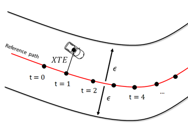
Note that this task is not so trivial. Even if we manually condition the vehicle speed at certain positions x, y of the road to achieve a certain value (for example, applying if/else over the speed along the reference trajectory), we cannot guarantee that this is the best option and it will require a long time of trials and errors until finding the best fit. Furthermore, every time the reference path changes, we will need to do everything again and again. So, how can we efficiently automate this task?
To answer this question, first check that the proposed problem clearly fits a Markov Decision Process (MDP):
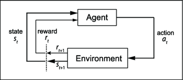
Where, under the trajectory environment, the AGV can represent the Agent, the action is based on selecting a certain speed and the states are the current vehicle positions x,y. The reward can be a function of the cross-track error: If the AGV surpass a certain threshold, it will be penalized.
To solve this simple MDP model, we can use Q-learning, one of the most popular RL algorithms in the current literature. You can find more information about the Q-learning at [4].
So, let’s model our Q-learning to find how to optimize the AGV speed according to the path. We need to define the state/action space and the rewards, as following:
- State space: We propose a discrete state space, in which both x and y coordinates of the planned path are sampled by 10 m spacing. We also include in the observation space the instantaneous XTE. In more details, there are 11 samples for x axis (from 0 to 110 m), 6 samples in y axis (from -40 to 20 m) and 4 samples for the XTE (from 0 to 2 m) sliced in pieces of 0.5 m each. This will result in a total of 264 states (11x6x4).
- Action Space: The proposed algorithm for each step must decide between two actions: increasing or decreasing the AGV target speed by 1 km/h.
- Rewards: The AGV will be penalized by -1 reward for each step taken until complete the planned path. Moreover, it will be punished by -1000 in case of the XTE surpass 1.5 m.
The model definition is relatively arbitrary, so feel free to try different model formulations, such as more resolution at the state space, or different reward values.
So, now let’s train our model. We are using a Q-Learning episodic approach with learning rate = 0.2, discount factor = 0.85 and exploratory rate of 0.01. The Figure below shows mean average over 100 epochs:
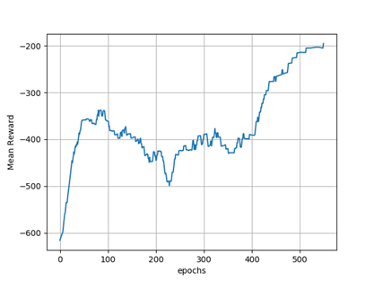
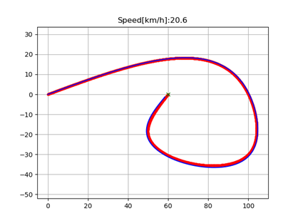
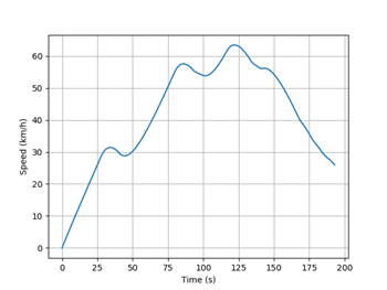
We can note that after 500 epochs, the algorithm converged to higher reward values. We stopped the training after -200 was reached. Actually, it is possible to improve even more this performance, but it also comes with a cost of better hyperparameters tuning (learning rate, exploratory rate, etc.).The Figure 1 and 2 below show the result of vehicle path following and speed, respectively, after the training. Check how the speed was adapted throughput the trajectory. When the vehicle started to approximate the sharp curve at the end of the path, it learned to reduce its speed in order to keep the track error within the margin of 1.5 m, as previously established.
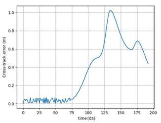
The Figure 3 below actually show the XTE variation through the path. It is interesting to check that the XTE starts increasing as it approaches the sharp curve in the path, but still respecting the maximum allowed XTE of 1.5 m.
4. Conclusions
In this article, we showed an example of controlling the speed of an autonomous vehicle by applying a Reinforcement learning technique. An intuition of autonomous vehicle control was provided, showing how the cross track error is impacted by vehicle speed. Therefore, the RL methodology help us to select an appropriate speed for the vehicle respecting the track error throughout the path.
5. References
[1] Brian Paden, Michal Cap, “A Survey of Motion Planning and Control Techniques for Self-driving Urban Vehicles”, 2016.
[2] Atsushi Sakai, “PythonRobotics: a Python code collection of robotics algorithms”, 2018.
[3] Sebastian Thrun, Mike Montemerlo, “Stanley: The Robot that Wonthe DARPA Grand Challenge”, 2006. http://robots.stanford.edu/papers/thrun.stanley05.pdf
[4] Andre Violante , “Simple Reinforcement Learning: Q-learning”, 2019.
