Collaborator: Pablo Ramirez Espinosa, post-doctoral researcher, Connectivity Section, Aalborg University
As presented in the previous post, GANs are a powerful framework for approximating the features distribution so as it is possible to generate fake samples that looks like real samples. In this post, in order to see some practical results of GANs approximation, we will present a toy example consisting in generating a bunch of real data that follows a Rayleigh distribution in order to see if the GAN framework can approximate the statistics of the Rayleigh distribution that was used for our real samples generation.
Rayleigh random variables generation
For the generation of our real samples, we are defining a matrix which is compounded of different realizations of Rayleigh random variables. Meaning then its PDF is:

For our study, we will generate these variables from the combination of two independent gaussian distributed random variables such as:

Being sigma = 1. Once this being said, we will generate a matrix compounded by m = 3600 samples of n = 1000 generated features that will be used for training both the generator and the discriminator. In this way the GAN will try to generate feature vectors compounded by 1000 Rayleigh distribution random variables.
GAN model implementation
For the implementation of the Generator and Discriminitor network, Python 3.6, Keras and Tensorflow have been used. The focus of this blogpost resides on looking at the interpretation of the results rather than in the pure implementation of the optimal neural network that will perform this task, so we will not cover in detail the implementation. However, in the reference section, one blogpost that have been used for the implementation of the current work is cited as extra information for the interest of the readers. The important thing to take into account in our current implementation, is the fact that we will be training and evaluating in batches (that is, small sets of the training set), so the computed loss and accuracy of both models are computed in every batch to track the training algorithm performance.
Training algorithm procedure
For the training procedure, the number of batches = 64 and the number of epochs = 10, meaning the number of iterations = 560. Then, the number of samples used in every iteration of real and fake data, will be half batch (32 real samples + 32 fake samples).
The procedure then will be:
- Get 32 randomly selected real samples
- Update the discriminator model weights
- Generate 32 fake samples
- Update the discriminator model weights
- Generate 32 fake samples
- Update the generator model weights via the discriminator’s error.
Then, for every iteration, we will keep track of the loss of both networks as well as the discriminator’s accuracy when predicting over real and fake samples.
Diagnosing GANs performance
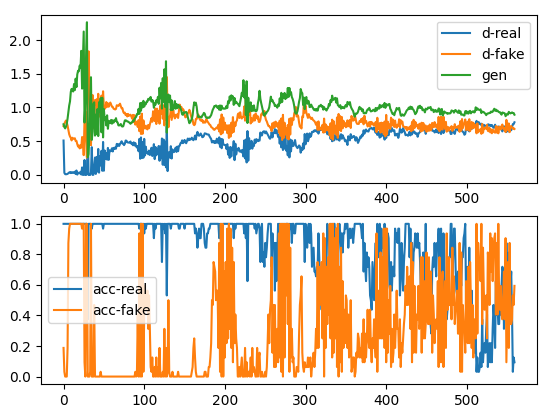
In order to check the convergence of our model, let’s take a look to the plots about loss and accuracy that were previously pointed out.

As we can see in the plots, convergence is occurring around > 460 iterations. In the first plot, the lines blue and orange corresponds to the loss achieved for real samples and fake samples with the discriminator network while the green one corresponds to the loss of the generator. The value of the losses are around 0.6, which makes sense taking into account what we saw in the last post, the loss optimal performance converges around -log(4), that is 0.6 if we take into account the quantity. Then, if we take a look into the second figure, the accuracy of the discriminator (on average, despite of the variance) is around 50% (discriminator forced to make coin flips decisions) when > 460 iterations. Sometimes, it can happen that there is a point in which the model the more iterations is trained, the worse performs so it starts diverging again. This means it is important to keep track of the perfomance into batches.
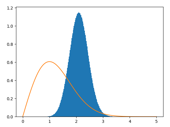
Finally, we have saved the model weights in different stages of the training procedure in order to generate fake samples. To have a visual comparison, we generate some fake samples and compute their respective histograms in order to compare it visually with the theoretical Rayleigh distribution from which real samples have been generated.

This plot corresponds to the histogram of generated fake samples when the training procedure was the 56 iteration. Related to the previous plot, it was expected that the approximation of the distribution would not be pretty accurate for this stage.

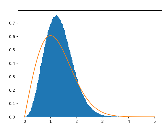
However, if we take a look at the iteration 448, the results now are better approximated. Although the mean of the distrubution is quite offseted yet.

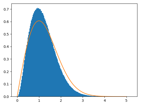
Finally, by taking a look at iteration 560, the approximation is way more accurate than the previous results. Note that, for a better performance, more real samples could be generated in order to make the algorithm to learn better the distribution. As well, some hyperparameters tuning could be addressed.
In order to have a quantitative measure of the performance, there is a common way addressed in literature which is named as Frechet Inception Distance (FID). Also, taking into account we are comparing two different distributions, the Cramer-Von Mises test could be addresed to compare the CDFs of both real and fake data and take a quantitative measure of how well the distribution is approximated. The evaluation of GANs performance in a quantitave manner will be addressed in the future in a new post.
Finally, to conclude this post, we will provide a comparison between the mean and standard deviation of both the real and fake data distribution.
Real distribution:
- Mean: 1.19
- Std: 0.58
Fake distribution:
- Mean: 1.25
- Std: 0.65
Note as mentioned previously that the results could be improved but still they are pretty accurate for our especific task.
References
- Goodfellow, I., Pouget-Abadie, J., Mirza, M., Xu, B., Warde-Farley, D., Ozair, S., … & Bengio, Y. (2014). Generative adversarial nets. In Advances in neural information processing systems (pp. 2672-2680).
- https://machinelearningmastery.com/practical-guide-to-gan-failure-modes/
- Cramér-von Mises test. Encyclopedia of Mathematics. URL: http://encyclopediaofmath.org/index.php?title=Cram%C3%A9r-von_Mises_test&oldid=44377
- Heusel, M., Ramsauer, H., Unterthiner, T., Nessler, B., & Hochreiter, S. (2017). Gans trained by a two time-scale update rule converge to a local nash equilibrium. In Advances in neural information processing systems (pp. 6626-6637).