Neural Autoregressive Models and Normalizing Flows

Estimation of probability density of high dimensional complex data distributions is a long-standing challenge in many different fields, including machine learning. Neural Autoregressive Density Estimation (NADE) is a method that estimates data distributions by modeling each term in the probability chain rule with a parameterized function [1].

(1) $\begin{align*}p(x_{1:d}) = p_\phi(x_1)\prod_{i=2}^D p_\phi(x_i|x_{1:i-1})\end{align*}$

The indices in (1) represent an arbitrary ordering of dimensions, i.e. $x_1$ , doesn’t need to be the first dimension of data. In this approach, we decompose the joint density into one dimensional conditional densities, where each conditional $p_\phi(x_i|x_{1:i-1})$ is a function of all the previous dimensions, e.g. a univariate Gaussian density, whose mean and variance are computed by deep neural networks (DNN).

$p(x_i|x_{i-1}) = \mathcal N(x_i|\mu_{\phi,i}(x_{1:i-1}), \exp(\alpha_{\phi,i}(x_{1:i-1}))^2)$

where $x_{1:0}$ is an empty sequence and its function is a constant.

The main contribution of NADE is its architecture that heavily ties the parameters of conditionals together, resulting in better learning and sample efficiency. The parameters, denoted by vector $\phi$ , are learned from data samples using Maximum Likelihood Estimation (MLE) or maximizing the Evidence Lower BOund (ELBO) for Variational Inference (VI). Unfortunately, likelihood evaluation in NADE from (1) is $\mathcal O(D)$ which is slow for high dimensions.

Although the chain rule in (1) holds for any distribution, the combination of the ordering in (1) and the selected densities for $p_\phi(x_i|x_{1:i-1})$ restricts the class of representable distributions with vanilla Neural Autoregressive models. For instance, we can’t model the 2d distribution in Figure (1 – left) using Gaussian conditionals and the ordering $p_\phi(x_1)p_\phi(x_2|x_1)$ , since distribution of $x_2$ may have up to two modes for a given $x_1$ . On the other hand, the ordering $p_\phi(x_2)p_\phi(x_1|x_2)$ would result in a more accurate model. As a rule of thumb, conditionals further ahead in the chain rule depend on more variables and can capture more complex relations with simple models with light tail and few modes. Densities with fewer dependencies, however, may require heavy tail and multimodal models.

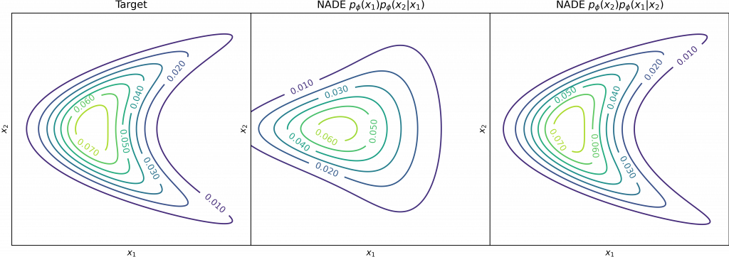Figure 1: (Left) Target distribution, (Center) NADE model trained with Gaussian conditionals and ordering $p_\phi(x_1)p_\phi(x_2|x_1)$ , (Right) same model trained with ordering $p_\phi(x_2)p_\phi(x_1|x_2)$ .

Therefore, many developed techniques focus on how to provide the correct inductive bias in the conditionals and ordering according to the structure of data (WaveNet, PixelRNN, PixelCNN, PixelCNN++). Alternatively, it is possible to stack multiple layers of NADE models and construct an ensemble of Neural Autoregressive estimators with deep and orderless NADE to compose complex distributions from the simpler ones.

Another important aspect of density estimators is whether they can efficiently generate samples from the model. In the case of Autoregressive models, we need to perform ancestral sampling

$x_i\sim p_\phi(.|x_{1:i-1})$

sequentially. This requires $\mathcal O(D)$ iterations which is considerably more expensive than the other deep generative models like Variational Auto-Encoders (VAE) and Generative Adversarial Networks (GAN). However, they are particularly interesting since they can provide an explicit likelihood function for model evaluation, comparison and selection.

Masked Auto-encoder for Density Estimation

Masked Auto-encoder for Density Estimation (MADE) is a popular architecture which implements the autoregressive dependencies in terms of connections of layers in a DNN. MADE an auto-encoder architecture is converted into an autoregressive model by applying a mask on the appropriate connections linking the high indices of the ordering to the conditionals of lower indices in each layer (Figure (2). Although, forward pass is still $\mathcal O(D)$ , we can enjoy the efficient parameter and computation sharing and speed boost from parallel computation of the conditionals with a single forward pass of the network [2].

Figure (2): Masking connections in 3 layer auto-encoder to construct an autoregressive model. Our ordering indices correspond to the input node numbers. To ensure autoregressive property, in each layer nodes are randomly indexed and the connections to larger numbers from the previous layer are removed from fully connected layers. Output nodes evaluate the parameters of the conditionals, which are then used to evaluate the joint likelihood of $x_{1:D}$ . 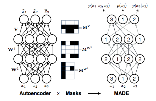[2]

Masked Autoregressive Flow

We can view the sampling process in NADE as an autoregressive transformation of samples from a base distribution. For simplicity, consider the Gaussian NADE model. To generate a sample $x_{1:D}$ , we first sample $D$ base variables $u_{1:D}$ independently for standard normal distribution $\mathcal N(0,1)$ . Then, we recursively apply the following transformation.

(2) $\begin{align*}x_i = u_i \exp(\alpha_{\phi,i}(x_{1:i-1})) + \mu_{\phi,i}(x_{1:i-1})\end{align*}$

Using MADE to evaluate $\mu_{\phi,i}(x_{1:i-1})$ and $\alpha_{\phi,i}(x_{1:i-1})$ as before, we can synthesize samples from the model distribution. Since each transformation in (2) is invertible, we can interpret the gaussian autoregressive model as a Normalizing Flow (NF) with the inverse transformation given by $u_{1:D} = T(x_{1:D})$ where

$T(x_{1:D})_i = T_{x_{1:i-1}}(x_i)= (x_i - \mu_{\phi,i}(x_{1:i-1}))\exp(-\alpha_{\phi,i}(x_{1:i-1}))$

and $T_{x_{1:i-1}}(x_i)$ is bijective in $x_i$ and all the $D$ base variables that generated data sample $x_{1:D}$ can be recovered in parallel. From the probability conversion rule, we know that

(3) $\begin{align*}p(x_{1:D}) = g(T(x_{1:D}))|J_T(x_{1:D})|\end{align*}$

where $g(.)$ is the standard normal density function, $J_T(.)$ is the Jacobian of $T$ w.r.t. $x$ and $|J_T(.)|$ is its determinant. Additionally, due to autoregressive transformation, Jacobian is triangular and can be evaluated in $\mathcal O(D)$ with parallelization even if $\mu_{\phi,i}(.)$ s and $\alpha_{\phi,i}(.)$ s are not invertible.

$J_T(x_{1:D}) = \prod_{i=1}^D \exp(-\alpha_i(x_{1:i-1}))$

Masked Autoregressive Flows (MAF) exploit this to evaluate the joint density (1) and train the model much faster than the vanilla Neural Autoregressive models [3]. This NF reformulation is only available for autoregressive models which have conditionals that we can reparameterize bijectively.

Inverse Autoregressive Flows

While the NF density formulation (3) speeds up likelihood evaluation for autoregressive models, sample generation remains essentially sequential in MAFs. This poses a problem particularly for VI where each training epoch requires samples from the approximate posterior model. We can solve this problem by inverting the MAF block and swapping the base and data variables. In Inverse Autoregressive Flows (IAF), we define $\mu_{\phi,i}(.)$ s and $\alpha_{\phi,i}(.)$ s as functions of previous base variables. Therefore, for sampling we get

(4) $\begin{align*}x_i = u_i \exp(\alpha_{\phi,i}(u_{1:i-1})) + \mu_{\phi,i}(u_{1:i-1})\end{align*}$

which can be evaluated in parallel for all the dimensions [4].

Speeding up the sample generation process comes at the cost of sequential likelihood estimation. IAF uses MADE architecture to implement the inverse transformation.

$u_i = (x_i - \mu_{\phi,i}(u_{1:i-1}))\exp(-\alpha_{\phi,i}(u_{1:i-1}))$

Similar to likelihood estimation in MAF, we can use the conversion rule to evaluate the joint density, since the Jacobian of transformation defined by (4) is triangular.

Coupling Layers

Coupling Layers where first introduced in NICE [5] and further developed in RealNVP [6], in order to perform both sampling and likelihood estimation without the sequential (MADE) transformations. In these transformations, a subset of base variables indexed by $d\subset \{1, ..., D\}$ are set as the reference and are passed directly to the output space, while the the rest of the base variables (indexed by $\bar d=\{1,...,D\}\setminus d$ ) are translated and scaled according to these references, i.e. using vector notation

(5) $\begin{align*}x_d &= u_d\\ x_{\bar d} &= u_{\bar d} \odot \exp(\alpha_\phi(u_d)) + \mu_\phi(u_d)\end{align*}$

for $\alpha_\phi:\mathbb R^{|d|}\to \mathbb R^{|\bar d|}$ and $\mu_\phi:\mathbb R^{|d|}\to \mathbb R^{|\bar d|}$ . The affine transformation in (5) can be replaced with a more complex transformation of $u_{1:D}$ as long as the transformation remains bijective in $u_{\bar d}$ and has a trivial Jacobian determinant.

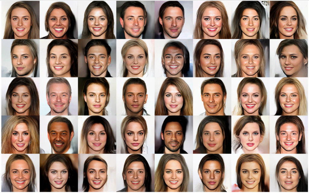
In coupling layer, the first $|d|$ conditionals of the chain rule (1) are modeled with independent marginal densities, while the rest only depend on $|\bar d|$ fixed indices from the previous variables, reducing the capacity of the autoregressive model. In particular, the theoretical results that prove universal representation of arbitrary differentiable and positive probability density function with bijectors relies on approximation of all the conditionals in (1) [7]. However, stacking many coupling layers with index permutation and batch normalization in between has been proven effective in modeling complex image distributions (Figure (3) and they are quite popular due to their efficient sample generation and exact likelihood estimation [8].

Figure (3): Generated samples from Glow with temperature 0.7 trained on 256×256 celeba dataset [8].

Discussion

In this study, we explained the connection between Neural autoregressive models and various Normalizing Flows and studied their advantages and efficiency in sample generation and likelihood evaluation. For a comprehensive review of NFs we refer the readers to [9].

Despite their success in lower dimensions, NFs couldn’t scale as well and GANs to “extreme” resolution images. Diagnosis of NFs in [10] shows that they transform simple data samples to high density regions (close to the mean) in the base distribution. This results in likelihood overestimation for out of distribution samples from less variant datasets. Moreover, with simple priors, NFs tend to become numerically nonivertible and allocate excessive density to threads connecting separated modes in the data distribution [11]. Due to these problems, sample generation is generally reported for tempered NF, where we transform samples of the base distribution with downscaled variance, trading-off sample diversity for its quality.

It is worth mentioning that NFs try to learn signal and noise distributions simultaneously using the same bijective transformation. This potentially requires a complex transformation. In comparison, bayesian VI uses posterior approximation to recover a low dimensional representation of the data samples and separate signal from the noise. The connection of NFs with bayesian VI is studied in [5]. Most DNN based VI methods suffer from blurred samples with low quality and unknown approximation gap. However, recently, Diffusion Probability Models achieved a new record for image compression and visual scores showing all you need is a very deep model and a posterior approximator which asymptotically inverts the generative process. One of the remarkable properties of NFs is that we can perform gradient based optimization with constant memory consumption. Because the gradient computation can use the inverse transformation to evaluate the activation values of each layer as in RevNets. Therefore, a very deep variational NF with controlled gradient flow may soon overcome all these problems and become the new state-of-the-art generative model.

References

[1] Uria, Benigno, et al. “Neural autoregressive distribution estimation.” The Journal of Machine Learning Research 17.1 (2016): 7184-7220.

[2] Germain, Mathieu, et al. “Made: Masked autoencoder for distribution estimation.” International Conference on Machine Learning. PMLR, 2015.

[3] Papamakarios, George, Theo Pavlakou, and Iain Murray. “Masked autoregressive flow for density estimation.” arXiv preprint arXiv:1705.07057 (2017).

[4] Kingma, Diederik P., et al. “Improving variational inference with inverse autoregressive flow.” arXiv preprint arXiv:1606.04934 (2016).

[5] Dinh, Laurent, David Krueger, and Yoshua Bengio. “Nice: Non-linear independent components estimation.” arXiv preprint arXiv:1410.8516 (2014).

[6] Dinh, Laurent, Jascha Sohl-Dickstein, and Samy Bengio. “Density estimation using real nvp.” arXiv preprint arXiv:1605.08803 (2016).

[7] Bogachev, Vladimir Igorevich, Aleksandr Viktorovich Kolesnikov, and Kirill Vladimirovich Medvedev. “Triangular transformations of measures.” Sbornik: Mathematics 196.3 (2005): 309.

[8] Kingma, Diederik P., and Prafulla Dhariwal. “Glow: Generative flow with invertible 1×1 convolutions.” arXiv preprint arXiv:1807.03039 (2018).

[9] Nalisnick, Eric, et al. “Do deep generative models know what they don’t know?.” arXiv preprint arXiv:1810.09136 (2018).

[10] Papamakarios, George, et al. “Normalizing flows for probabilistic modeling and inference.” arXiv preprint arXiv:1912.02762 (2019).

[11] Cornish, Rob, et al. “Relaxing bijectivity constraints with continuously indexed normalising flows.” International Conference on Machine Learning. PMLR, 2020.

June 24, 2021

Research

neural autoregressive models, normalizing flows