As you may have guessed from its name, Hierarchical Reinforcement Learning (HRL) is a family of Reinforcement Learning algorithms that decompose the problem into different hierarchies of subproblems or subtasks, and the higher-qlevel tasks invoke the primitive lower-level tasks. The goal of HRL is to learn a multilayer policy to perform control at different levels of temporal abstraction.
Unlike flat RL, the agent can now choose either macro actions (consisting of sequences of lower-level actions) or primitive lower-level actions. Due to the hierarchy and passing the control among the layers the time between different macro actions may not always be the same. Fortunately, the Semi-Markov Decision Process (MDP), a generalization of MDP, can be applied to model a system with different elapsed time between actions.
HRL can effectively reduce the computational complexity of the overall problem by breaking it down into several simple subproblems and independently solving these small problems. The learning procedure can also be further accelerated by transferring the knowledge between different subtasks thanks to the generalization provided by HRL. On the downside, given the hierarchy constraints, in general, there is no guarantee that the decomposed solution provided by HRL is also an optimal solution to the original RL problem [1].
Hierarchical Reinforcement Learning
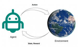
The figure below presents the general structure of an RL system, where the agent learns from interacting with the environment within an action-reward loop. At each time step, based on its observation from the environment, the agent takes action and receives the reward for the action taken and the new state.
Unlike the traditional RL, the HRL agent is provided with background knowledge about the decomposition of the environment, which can be given explicitly or learned through interaction with the environment. Like traditional RL, the agent’s goal is to learn the policy that maximizes the cumulative future rewards.
A simple environment is presented in the figure below to further discuss the motivation behind the problem decomposition in HRL.
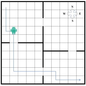
The figure shows a four room house with a gate between adjacent rooms, where a 10×10 grid quantizes the space in 100 cells. Each cell represents an individual state that the agent can occupy. The agent always starts from the most top-left cell, and the goal is to reach the most bottom-right cell. Suppose that the agent can sense the environment and find its “state,” i.e., the room that it occupies and its position in the room. In each step, the agent can take either one of the north, south, east, and west actions that move the agent’s state to the adjacent cells. The action that takes the agent to the wall leaves its location unchanged. The agent receives a -1 reward at each step, and the goal is to reach the final state in the shortest time. Conventional flat RL needs to store 400 Q-values (100 states and four actions for each state) to solve this problem effectively. Another approach for solving this problem is to decompose the state space into two hierarchies of levels: at the higher level, a master agent learns which room to go to, while at the lower level, the worker agents learn how to find the path to the gate of the room chosen by the higher-level policy. The agent’s position inside each room is abstracted to the higher-level agents as it looks at the room as a whole and aims to navigate between the rooms. Once the master agent learned the optimal policy, each “macro” action (choosing the next room to go to) will invoke and pass the control to the worker agent to move toward the chosen room’s gate. The actions of the master agent are temporally extended because once they are performed they will persist until the agent leaves the current room and enters the new one. The worker agent will then pass the control back to the master to choose the next room. Here the master agent requires only 8 Q-values (4 rooms and two actions, corresponding to the two exit gates from each room) to store. The worker agents are also required to store the Q-values for their own state-space (e.g., the room occupied). Assume a given higher-level policy chooses to enter the rooms, as shown in the figure. In this case the agents need to store 8, 100, 100, and 80 (in total 288) Q-values, which is comparatively smaller than the values for flat RL agent. This gap goes even higher by increasing the scale of the problem. Also, having multiple similar sub-tasks will help the agents to accelerate the learning process by sharing the knowledge between worker agents.
Different Hierarchical Reinforcement Learning Models
Here we will review the most well known architectures presented for the HRL problems. We will start with some classic models from the 1990s and then will expand the discussion to more advanced methods that relays on deep neural networks.
The Option Framework
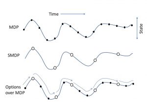
The options framework [2] is a well known formulation for HRL that was introduced by Sutton et al. in 1999. This framework uses the SMDP to model the RL agent. The framework defines the concept of option as a generalization of actions that lets the agent choose between the macro and primitive actions. More formally, an option is defined by a triple t=<Io,πo,βo>, where Io is the initiation set, πo: S×A→[0, 1] denotes the option’s policy and βo:S→[0, 1] defines the termination condition. By observing a new state, the agent checks whether it belongs to the initiation set Io, in which case option o is started. The policy πo then takes control and chooses the actions to be taken. At the end of each step βo is checked for termination condition, and, if true, the control goes back to the global policy. The algorithms following the options framework with both primitive actions and options are proven to converge to the optimal policy. The figure below shows how the options framework could manage actions and states with different temporal lengths.
Hierarchies of Abstract Machines
Hierarchical Abstract Machine (HAM) [3] defines the subtasks employing stochastic finite estate automata named abstract machines, where each machine can call other machines as a subroutine. HAM defines two types of machines: action states that determine the action to be taken in a certain MDP state and choice states that select the next machine state with nondeterministic actions. More formally, an abstract machine can be defined by the triple t=< μ, I, δ >, where μ is the finite set of machine states, I denotes the stochastic function that maps the MDP states to machine states, and δ represents the next-state function that receives the MDP and machine states and returns the next machine states.
Feudal Reinforcement Learning
Feudal reinforcement learning [4] defines a hierarchy of control, where a level of managers controls sub-managers and at the same time is controlled by higher level super-managers or workers. Higher layer managers assign goals to the workers that are rewarded by performing actions and reaching the goals. Feudal learning is based on two concepts: Information and Reward hiding. Information hiding implies that managers observe the environment at different resolutions and only need to know the state of the system at the granularity of their own choice of tasks. Reward hiding means that the reward given to a sub-manager is based on satisfying the sub-goals assigned by the manager, which leads the sub-managers to learn a policy that satisfies the higher level managers.
MAXQ
MAXQ [5] is another formulation for HRL that obtains a hierarchy of tasks by recursively decomposing the value function of the original MDP into value functions of smaller constituent MDPs. Each smaller MDP essentially defines a subtask that can further decompose unless it is in a terminal state. The decomposition of Q-values is done as Q(p,s,a) =V(a,s) + C(p,s,a). V(a,s) is the expected reward by taking action a in states, and C(p,s,a) is the expected reward for the overall problem after the subtask p is terminated. Here the action a can be a primitive action or a sequence of actions.
Feudal Networks
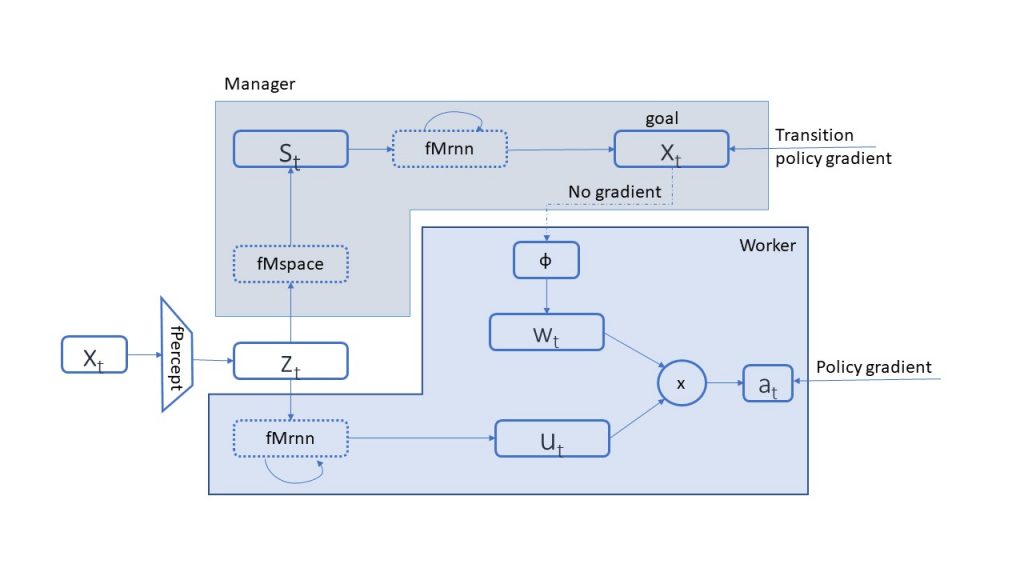
Inspired by Dayan’s Feudal model for HRL, DeepMind introduced the FeUdal Networks [6] in 2015. They presented a modular architecture consisting of two independent Neural Networks (NNs) that operate as manager and worker. The model is shown in the figure below, where both the manager and the worker receive a representation of the observation z. The manager creates a different latent state t with a higher dimension d and passes it to a recurrent NN (fMrnn), which defines the subgoal gt for the worker to achieve. On the other side, the worker receives the assigned sub-goals as well as the observation representation z and returns the optimal actions to take. The actions are taken in such a way that satisfies the sub-goals defined by the manager.
Option-Critic Networks
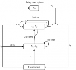
The Option-Critic architecture [7] extends the Options framework, where the options are not predefined and can be started from any state. The internal policies and the termination conditions can also be learned employing the gradient theorem as described in [8]. As the figure below shows, two levels of policies are defined. The policy over options chooses among options in each step and leaves the control to the sub-policy of the chosen option until it returns a terminated condition. The Option-Critic architecture is based on actor-critic approach, where an actor network tries different actions and a critic network evaluates the performance of the chosen action and gives feedback to the actor. The actor consists of the local policy, termination functions, and the policy over options, while the critic keeps QU, the values of the actions taken in different state-option pairs, and AΩ, the advantage function over options.
Conclusion
The potential of HRL to reduce the complexity of a big problem by dividing it into several simple subproblems and independently learning the optimal solution for each sub-problem makes it very interesting for researchers. This behavior is inspired by human’s approach to solving complex problems hierarchically. HRL is still in its infancy and has a long way to go before applying it in real world use cases.
[1] B. Hengst, Hierarchical Reinforcement Learning, pp. 495–502. Boston, MA: Springer US, 2010.
[2] Sutton, R.S., Precup, D. and Singh, S., 1999. Between MDPs and semi-MDPs: A framework for temporal abstraction in reinforcement learning. Artificial intelligence, 112(1-2), pp.181-211.
[3] Parr, R. and Russell, S., 1998. Reinforcement learning with hierarchies of machines. Advances in neural information processing systems, pp.1043-1049.
[4] Dayan, P. and Hinton, G.E., 1993. Feudal reinforcement learning. NIPS’93 (pp. 271–278).
[5] Dietterich, T.G., 2000. Hierarchical reinforcement learning with the MAXQ value function decomposition. Journal of artificial intelligence research, 13, pp.227-303.
[6] Vezhnevets, A.S., Osindero, S., Schaul, T., Heess, N., Jaderberg, M., Silver, D. and Kavukcuoglu, K., 2017, July. Feudal networks for hierarchical reinforcement learning. In International Conference on Machine Learning (pp. 3540-3549). PMLR.
[7] Bacon, P.L., Harb, J. and Precup, D., 2017, February. The option-critic architecture. In Proceedings of the AAAI Conference on Artificial Intelligence (Vol. 31, No. 1).
[8] Sutton, R.S., McAllester, D.A., Singh, S.P. and Mansour, Y., 2000. Policy gradient methods for reinforcement learning with function approximation. In Advances in neural information processing systems (pp. 1057-1063).