Kernel Ridge Regression

This article aims to introduce and clarify kernel ridge regression. To do so, it is necessary to derive a simple formula: the orthogonal projection formula. The reason is that, to understand kernel ridge regression, we need to understand how linear regression works, but the whole theory of linear regression relies on the solution of the following question: what is the projection of a vector on a vector .

We assume that the vectors live in finite dimensional Euclidean space and vectors are always column vectors.

Projection of vector on vector

First, let’s consider simple case of projection vector on vector in -dimensional Euclidean space. Figure 1. Illustrates this scenario. Vector we want to find is , which is the projection of on .

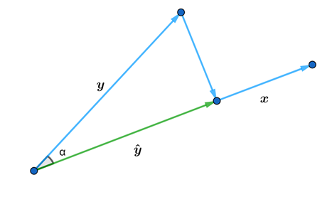
First of all, notice that the projection vector is just a “rescaled version” of the vector , that is . How much we should “rescale” depends on two things: (i) How long the vectors and are. (ii) Most importantly mutual arrangement of the vectors and ! Both of the points above can be formalized by the notion of scalar product (central object of this article). In Euclidean space scalar product is defined as follows (you may recognize the low of cosines)

   

To see why the scalar product carries some information about mutual arrangement of the vectors, consider two extreme scenarios: (1) When and are orthogonal to each other or (2) they have the same direction. In the first case, the scalar product is zero since . For the second case, scalar product achieves the maximum value, which is the product of the length of vectors.

Problem 1. How is this fact related to the Cauchy-Schwarz inequality?

Problem 2. Denoting by and Y random vectors with realizations and correspondingly, what is the relationship between sample correlation of and and the formula

   

Going back to the projection formula, we have to find scale factor in . Notice that dividing by gives us the vector with the same direction and the length 1 (this procedure called normalization). If we replace with in then the problem of finding is equivalent to the problem of finding the length of , so By the definition of we have , using the formula from Problem 2 gives us .

   

If the vector has the length one, the formula above can be simplified as follows

   

Let us denote the operation by , so the operation does the projection of any vector to the given vector of unit length. Now observe that the operation is linear in the second argument

   

and maps vector to vector, therefor it can be represented as a matrix, that is there exists matrix , called projection matrix such that

   

Problem 3. Show that the matrix is nothing more than (Hint: .)

Problem 4. Show that , where

To summarize, matrix acting on the vector projects it onto the unit length vector . For general we have to normalize it by its length , so

   

The following observation will be important in the future. For the unit length vector

   

It allows us to write projection in terms of linear combination of product .

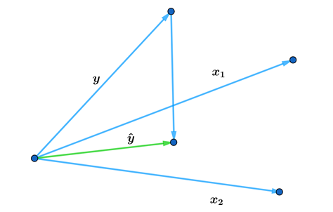
Projection of vector on space

What about more general scenario when we want to project not on the one vector, but on the space spanned by bunch of vectors Figure Illustrates this scenario when and space is three-dimensional.
Surprisingly the formula for the projection in general case is very similar. What we have to do is just replace vector with matrix whose columns are the vectors spanning the subspace we want to project on

   

When the vectors are orthonormal, that is when , then and

   

Equality above means that the projection on the space spanned by orthonormal system is just a sum of projections on individual vector.

Problem 5. What does it mean in terms of linear regression? (Hint: In linear regression vectors are inputs (features), orthogonality just means that they are uncorrelated. When the inputs are uncorrelated, they have no effect on each other’s parameter estimates in the model.)

As was discussed for one vector case, the projection is just rescaled (reweighted) version of the vector where we are projecting, with the weight given by a scalar . Same is true for the projection on the space spanned by multiple vectors, what changes is that we have to reweight each according to the component of the weighting vector . It means that

   

Notice that the projection of into always exists whenever . In general case it can happen that for all , but may not be defined.

Problem 6. When does it happen?

This problem can be solved easily by adding a positive constant to the diagonal of before inversion. Even if is not invertible is well defined for . Procedure just described is known as Tikhonov regularization in literature. This motivates us to define regularized projection matrix

   

and corresponding projection vector

(1)  

where . \section{Kernel ridge regression} Now it’s time to talk about kernel ridge regression. To do so it’s more natural to talk about rows (observations) of the matrix rather then columns. Let’s denote them by , so . First we need to rewrite identity (1) in terms of row vectors of . To do so we need the following identity

   

Problem 7. Show that the identity above is true. Hint: .

Using this identity, we can write

   

where As one can see, to calculate projection you only need to know scalar product of the observations. It means that all you need to know is similarity measure of two input observations. In the derivation above we used ordinary scalar product for that. Main idea behind kernel ridge regression (and other kernel based methods SVM, GP,… ) is to replace the scalar product everywhere in the representation above by the scalar product of the form

   

where is some symmetric, positive definite function called \textit{kernel}. For instance, the kernel

   

known as a linear kernelgive us back linear regression. In practice non-linear kernels are more popular. Example of non-linear kernel is polynomial kernel

   

Another popular kernel is exponential kernel

   

Problem 8. Why do we require kernel to be symmetric and positive definite? Do the examples of kernels defined above satisfiy this requirement? Can you give other examples of kernels?