Grassmann Manifolds - Subspace Comparisons

In this article we will review the basic concepts related to Grassmann Manifolds and how they are applied in subspace comparison. The original motivation for this post can be found in the field of clustering of multi-antenna wireless communication [1], which is the focus of my research in the context of the Windmill project.

Quick recap on subspaces

Principal angle between two subspaces — Principal angle $\theta$ between two subspaces $\mathcal{X}, \mathcal{Y}$ .

Before going into further details regarding manifolds and how they can be used in subspace comparison, let us first recall some concepts of linear algebra. We start by reviewing the concept of vector spaces. In short, a vector space $\mathcal{V}$ is normally defined by a set of vectors $\mathcal{W} = \{w_1, \dots, \w_N\}$ together with a field $\mathcal{F}$ (a collection of scalars). These vectors may be added together or multiplied by the elements of this field to describe new vectors. Note that in this sense the zero vector has to be defined in this space. Moreover, the span of a set of vectors is defined as the set of all possible linear combinations of this set, and the dimension of a vector space is the number of vectors in its smallest spanning set.

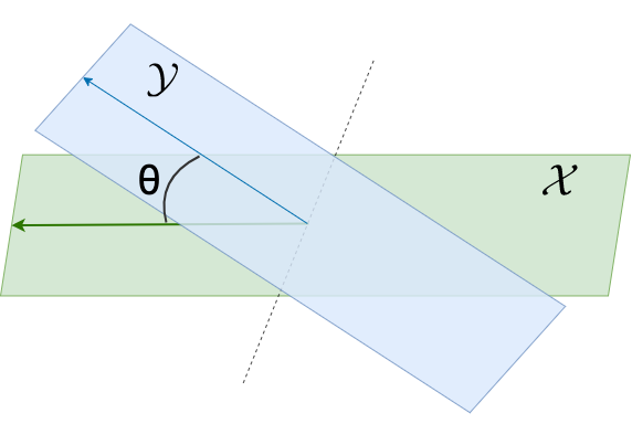
Similarly to how one would define angles between vectors, one can also define angles between spaces (or subspaces). In this case these angles are called principal angles.

Consider two subspaces $\mathcal{X}, \mathcal{Y}$ in the n-dimensional eucledian space $\mathbb{R}^n$ of dimensions $p$ and $q$ , respectively. The $m = \mathrm{min}(p, q)$ principal angles $0 \leq \theta_1 \leq \theta_2 \leq \dots \leq \theta_{m} \leq \pi/2$ between these subspaces, and their corresponding principal vectors, are defined recursively by
$\mathrm{cos}(\theta_k) =\underset{\substack{ \mathbf{x} \in \mathcal{X} \ \mathbf{y} \in \mathcal{Y}}}{\max } \hspace{0.2em}|\mathbf{x}^\mathrm{T} \mathbf{y}| = |\mathbf{x}_k^\mathrm{T} \mathbf{y}_k|$
subject to
$||\mathbf{x}|| = \mathbf{y} = 1, \hspace{2em} \mathbf{x}^\text{H}\mathbf{x}_i = 0, \hspace{2em} \mathbf{y}^\text{H}\mathbf{y}_i = 0, \hspace{2em} i = 1, \dots, k-1$
The vectors $\{x_1, \dots, \x_m\}$ and $\{y_1, \dots, \y_m\}$ are the principal vectors. We will also define $\Theta = \{\theta_1, \dots, \theta_k, \dots, \theta_m \}$ as the collection of all principal angles between these vectors.

As we will discuss later, the principal angles induce several distance metrics on the Grassmann manifold. In practice, the principal angles between $\mathcal{X}$ and $\mathcal{Y}$ can be computed from the singular value decomposition (SVD) of their orthonormal bases.

Let the columns of $\mathbf{X} \in \mathbb{R}^{n\times p}$ and $\mathbf{Y} \in \mathbb{R}^{n\times q}$ form the orthonormal bases for the subspaces $\mathcal{X}$ and $\mathcal{Y}$ respectively. Then we have that the singular values of $\mathbf{X}^\mathrm{H}\mathbf{Y}$ correspond to the cosine of the principal angles $\mathbf{\Theta}$ .

Grasmann Manifolds

Example of Grassmann Manifold $\mathcal{G}(1,3)$ . Extracted from [2].

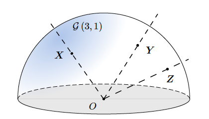
The Grassmannian manifold $\mathcal{G}(K, N)$ refers to the $N$ -dimensional space formed by all $K$ -dimensional subspaces embedded into a $N$ -dimensional real (or complex) Euclidean space. Let’s take the same example as in [2]. Think of embedding (mapping) lines that pass through the origin in $\mathbb{R}^2$ into the 3-dimensional Euclidean space. Note that these lines are one-dimensional entities, i.e., can be described by a single value. Now think of a smooth geometry (semi-sphere) that intersects all these lines. The points laying on this semi-sphere are the points in the Grassmannian manifold $\mathcal{G}(3, 1).$ One often defines real Grassmannian manifolds as

$\mathcal{G}(K,N) = \{ \mathrm{span}(\mathbf{X}): \mathbf{X} \in \mathbb{R}^{N\times K}, \mathbf{X}^\mathrm{H}\mathbf{X} = \mathbf{I}_k \}$

to represent the set of $K$ -dimensional subspaces embedded in a $N$ -dimensional Euclidean space. According to this notation, the Grassmannian $\mathcal{G}(K,N)$ can be seen as the manifold built of the symmetric projections matrices of size $N\times N$ and rank $K$ [2,3].

Distance Measures

As mentioned above, the distance between subspaces can be geometrically characterized by their principal angles. And, of course, there is a relationship between the principal angles of two subspaces and their distance in the Grassmann manifolds. In fact, the principal angles induce several distance metrics on the Grassmann manifold $\mathcal{G}(K, N)$ , which in turn provides a topological structure to the set of all $K$ –dimensional subspaces in a $N$ –dimensional space [1,2].

For instance, let’s consider the squared projection-Frobenius distance

$d^2_\text{PF}(\mathbf{X}_k,\mathbf{X}_j) = \sum_{i=1}^N \sin^2(\theta_{k,j}(i)) = \ N - \mathrm{tr}({\mathbf{X}}_k {\mathbf{X}}_j)$

where $\mathrm{tr}(\cdot)$ denotes the trace of a matrix. This similarity represents how far two subspaces are based on the cosinus of their principal angles. Similarly, one can also relate the principal angles to the pseudo-determinant (product of non-zero eigenvalues) of the product ${\mathbf{X}}_k {\mathbf{X}}_j$ , in which case we end up with the squared Fubini-Study distance that can be described by

$d^2_\text{FS}(\mathbf{H}_k,\mathbf{H}_j) = \prod_{i=1}^N \cos^2(\theta_{k,j}(i)) = \mathrm{pdet}({\mathbf{X}}_k {\mathbf{X}}_j)$

, where $\mathrm{pdet}(\cdot)$ denotes the pseudo-determinant. The main advantage of $d^2_{\text{PF}}$ with respect to other metrics is the fact that it can be computed without the need for eigendecompositions.

Note that these are not the only distances that one can define between points in the Grassmann manifold. There are several other measures, and the table below makes a summary of the four most used ones. For further details in these metrics we refer the reader to [3].

Name	Based on Principal Angles $(\theta_{k,j})$	Based on Bases $({\mathbf{X}}_k, {\mathbf{X}}_j)$
Projection-Frobenius	$\sum_{i=1}^N \sin^2(\theta_{k,j}(i))$	$N - \mathrm{tr}({\mathbf{X}}_k {\mathbf{X}}_j)$
Fubini-Study	$\prod_{i=1}^N \cos^2(\theta_{k,j}(i))$	$\mathrm{pdet}({\mathbf{X}}_k {\mathbf{X}}_j)$
Arclength	$\sum_{i=1}^N \theta_{k,j}(i)$	–
Spectral Distance	$\min_i \sin(\theta_{k,j}(i))$	–

Table: Distances in Grassmannian Manifolds for Equidimensional Subspaces

Comparing Manifolds of Different Dimensions

So far we have primarily focused on quantifying the alignment (distance) of two equidimensional subspaces. However, in real-world applications [1,2,8,9], it is very common to encounter scenarios where the comparison of subspaces with distinct dimensions is made necessary. With that in mind, distinct research groups have come up with proposals for computing a distance between subspaces of different dimensions — containment gap [4], symmetric direction [5], distance and Schubert varieties [6]. However, in such approaches, one often needs to perform an extra step (normally involving a Monte Carlo simulation) in order to account for statistical significance of the comparison. In order to overcome this and other difficulties, we have recently proposed [1] a purely statistical comparison mechanism based on the asymptotic behaviour of the projection-Frobenius distance. The table below summarizes this and other methods proposed in the literature.

	Measure between $\mathbf{X}_j, \mathbf{X}_k$ ( $K_k < K_j$ )	Idea behind it
Containment Gap	$\underset{\mathbf{x}_k\in \mathbf{X}_k}{\max}~\underset{\mathbf{x}_j\in \mathbf{X}_j}{\max}\frac{\|\| \mathbf{x}_k - \mathbf{x}_j \|\|}{\|\|\mathbf{x}_k\|\|}$	Normalising subspaces distance based on the smaller subspace
Symmetric Direction	$\max(k, j) - \sum^{K_k}_{i=1}\sum^{K_j}_{j=1} (\mathbf{x}_k^\text{T}\mathbf{x}_j)^{2}$	Frobenius norm based solution
Schubert Varieties	$d(\mathbf{X}_k, \mathbf{X}_k)^2 + c_{*}\|K_k - K_j\|^2$	Compare subpaces in the doubly infinite Grassmannian $\mathcal{G}(\infty, \infty)$ . See [6] for details in $c_{*}$ , which depends on the metric of choice $d(\cdot, \cdot)$
Asymptotic behavior	$\frac{ d(\mathbf{X}_k, \mathbf{X}_k)^2 - \eta_{k,j}}{\sigma_{k,j}}$	With $\eta_{k,j}$ and $\sigma_{k,j}$ being the first and second-order statistics of metric $d_{k,j}(\cdot, \cdot)$

Table: Distances between different Grassmann Manifolds

References

[1] R. Pereira, X. Mestre and D. Gregoratti, “Subspace Based Hierarchical Channel Clustering in Massive MIMO,” GLOBECOM 2021 – 2021 IEEE Global Communications Conference, 2021, pp. 1-6. (in press)
[2] Zhang, Jiayao, et al. “Grassmannian learning: Embedding geometry awareness in shallow and deep learning.” arXiv preprint arXiv:1808.02229 (2018).
[3] Edelman, A., Arias, T. A., and Smith, S. T. (1998). The geometry of algorithms with orthogonality constraints. SIAM journal on Matrix Analysis and Applications, 20(2), pp. 303-353.
[4] C. A. Beattie, M. Embree, and D. C. Sorensen, “Convergence of polynomial restart Krylov methods for eigenvalue computations,” SIAM review, vol. 47, no. 3, pp. 492–515, 2005.
[5] X. Sun, L. Wang, and J. Feng, “Further Results on the Subspace Distance,” Pattern recognition, vol. 40, no. 1, pp. 328–329, 2007.
[6] K. Ye and L.-H. Lim, “Schubert Varieties and Distances between Subspaces of Different Dimensions,” SIAM Journal on Matrix Analysis and Applications, vol. 37, no. 3, pp. 1176–1197, 2016.
[7] Britannica, The Editors of Encyclopaedia. “Vector space”. Encyclopedia Britannica, 19 May. 2011, https://www.britannica.com/science/vector-space. Accessed 18 October 2021.
[8] Keng, Brian. “Manifolds: A Gentle Introduction”. bjlkeng.github.io/posts/manifolds/. Accessed 18 October 2021.
[9] Bendokat, T., Zimmermann, R., & Absil, P. A. (2020). A Grassmann manifold handbook: Basic geometry and computational aspects. arXiv preprint arXiv:2011.13699.

October 14, 2021

Research

Grassmann Manifolds, linear algebra, math, phd

Grassmann Manifolds – Subspace Comparisons