The aim of this post is to provide a general understanding of GANs and a discussion of the potential of this concept. This post is based on the paper which introduced the framework for generative model estimation. In order to address this matter, the post is going to be divided into three main contributions as follows:
- General explanation of GANs
- Formal description
- Theoretical proofs to analyze the potential of this type of networks.
What does Generative Adversarial Networks mean?
We are going to provide an overview of each of the terms that constitute this concept with the aim of understanding it from a high level perspective.
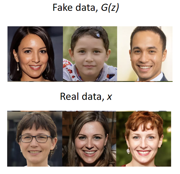
The term generative refers to the creation of new data samples that look like the training data.

At a first glance, I am sure no one could tell this image is actually fake, that is, this person does not exist. The ability of GANs resides in learning perfectly how data is distributed (pixel values in this especific case) when trained into a stable stage. We will dive into this later in the post.
The term adversarial is actually explained as an adversarial game in which a detective and a counterfeiter are involved.
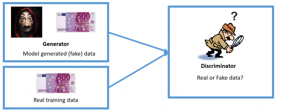
In this case, the goal of the counterfeiter (generator) is to create fake 500 euros bills to fool the detective (discriminator) while the discriminator’s task is to determine if the data taken as input is either real or fake. When the training process starts, both the discriminator and the generator have no idea of how real data looks like, hence the generator just outputs some random noise while the discriminator is forced to make random decisions. Along the process, we keep track of who is properly performing and who is not. In this way, if the discriminator is really easily determining if the data is real or fake, we will be updating the generator to improve its performance, and, in the opposite case, we will be updating the discriminator. When the training process converges, the discriminator is forced to make coin flip decisions because it cannot distinguish between the two types of data. This is because the generator has learnt how to create fake samples that look exactly like real samples, or in other words, the probability distribution of fake samples matches the probability distribution of real samples. The latter idea is going to be further developed in the last section.
The term nets refers to neural networks. Both the generator and the discriminator are implemented as neural networks. However, the first question to address is: why are neural networks used for this matter? The reasons for this are twofold:
- Universal approximators. Deep neural networks have been proved to be suitable as universal function approximators. Imagine how difficult is to model the probability distribution of pixel values along an image to conform a person’s face.
- Backpropagation algorithm. There are already well known optimization algorithms that perform really well in deep neural networks tasks.
Formal description of GANs
As it was previously stated, the GAN framework is compounded by two neural networks: the discriminator and the generator.
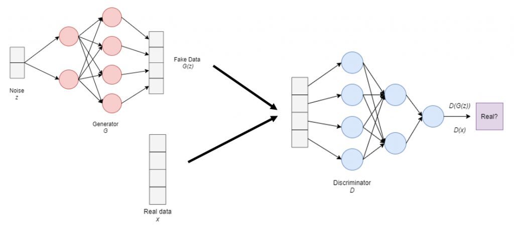
Let’s unwrap this image step by step. Firstly, we have the Generator denoted as G which takes as input some random noise, denoted as z. Then, the fake data is generated and denoted as G(z). Secondly, we have the real data, denoted as x. Take into account that the dimensions of the real and the fake data are identical, which is not a coincidence. Thirdly, we have the Discriminator, denoted as D, which takes as input either real or fake data and outputs the probability score of the taken input being actually a real sample. Then, when the input is a real sample, it is denoted as D(x) and when the input is a fake sample, as D(G(z)).
GANs cost function
Now, we are going to focus on the explanation of the GANs cost function described in the paper.

The cost function is compounded by two parts. The first part corresponds to the output of the discriminator when the input comes from the real data distribution, while the second one refers to its output when the input comes from the fake data distribution. If we take, for example, the first term, the calculation done is the expectation value of the log of the discriminator output when the input comes from the real data distribution. In other words, this means that we gather an amount of real data, compute the output of the discriminator, and then, we average the results. Same thing applies to the second term for the fake data.
What is the goal of the discriminator?

When the data is a real sample, the goal of the discriminator is to output a high probability score, which means that the real data sample taken as input was actually classified as a real sample.
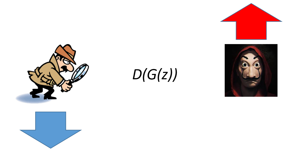
Then, when data is a fake sample, the adversarial game starts. The generator wants to fool the discriminator, meaning it wants this quantity to be as high as possible, while the discriminator wants to detect that it is fake, that is, it wants it to be as low as possible. However, if we used 1-D(G(z)) instead:
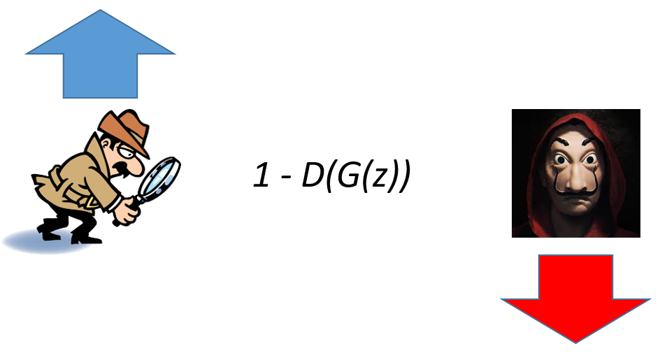
Now, the discriminator wants to maximize this quantity while the generator wants to minimize it. Once this being said and taking a look to our cost function:

In this way, the second term makes sense. The rewriting has allowed both opposite directions for the optimization process: the discriminator wants to maximize this entire quantity while the generator wants to minimize it.
Training algorithm
Once we are clear on the optimization objective, let’s take a look at the training algorithm described in the paper.
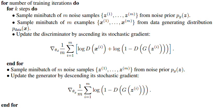
Firstly, the discriminator is updated because we want it to converge faster than the generator. In this way, for each training iteration, during k steps (they set it up to 1 and consider it as a hyperparameter):
- We gather m fake samples.
- We gather m real samples.
- We update the discriminator by ascending the gradient.
The expression this time is computed with respect to the parameters of the discriminator, by trying to maximize the whole expression.
Secondly, the generator is updated:
- We gather m fake samples.
- We update the discriminator by descending the gradient.
This time, we are computing with respect to the generator parameters. Note that the expression has removed the first term because real samples do not apply in the generator training procedure.
In a nutshell, this is how a GAN works and how it is trained. However, in the next section, the theoretical proofs presented in the paper are described for a better understanding of the potential of this framework.
Theoretical proofs: Perfectly matched distributions
The authors of this paper have proved that the minimum of the cost function is achieved if and only if the probability distribution of the fake samples matches the probability distribution of the real samples.
This means that the fake samples become identical to the real samples, therefore we are no longer capable of distinguishing if a sample is real or fake. The authors’ proofs have been developed in two parts that are being addressed in the next two sections.
Maximizing the Discriminator
The maximum of the cost function converges into a constant, concretely:

To explain this, we are rewriting again our cost function:

Although this time, we are writing the expectation values in their integral form:

If we take a look at the second term, we can perform a change of variable, so that we can directly integrate output over the generator instead of indirectly from the input noise variable. In this way, we now have a full expression which depends on just one variable x which represents data samples. If we want to maximize this expression over the whole integral in every single point, we would maximize the entire quantity. In every point of the integral, the function looks as follows:

If we compute the derivatives and set the expression to zero we can apply some calculus to find the extremum of the function. With some algebraic manipulations, we will end up having:
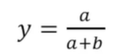
Then, by plugging in our concrete values:

We can see that the expression of the optimal discriminator is a simple relationship between the probability distributions. Also if the probabilities match:
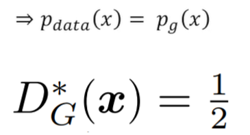
It is simple to see that in case the probabilities are identical, the expression of the optimal discriminator is 1/2. This makes intuitively sense because it means that the discriminator is forced to make coin flip decisions due to the real and the fake samples being identical.

Then, if we plug in this value in our cost function, we can obtain the aforementioned -log(4). However, the main two things to recap are the following:

The expression of the optimal discriminator is a simple relationship between the probability distributions and when they are equal, the cost function has a maximum, concretely -log(4).
Minimizing the Generator
The second part of the proof corresponds to the minimization of the cost function:

Now, we can plug in our previously commented expression to set an upper bound of the loss. Now, the definition of the KL Divergence is as follows:
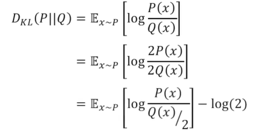
The KL Divergence is a measure of dissimilarity between two probability distributions. A more detailed explanation is beyond the scope of this post. It is useful for us because it allows us to rewrite our cost function as:

Then, one last definition should be included, which is the Jensen-Shannon Divergence:

Similar to the KL divergence, it measures the dissimilarity of two probability distributions but in this case, this divergence is symmetric. Again, a more detailed explanation is beyond the scope of this post. Then, by rewriting our cost function:

This -log(4) is the very same one that we were discussing before. Hence, to wrap up everything: which is the point of all this math?

This shows that for an optimal discriminator, the generator tries to minimize this quantity. The first term is a constant, so nothing can be applied to minimize it and we have to focus on the second term. By definition, the minimum of the JSD is 0 when the probability distributions are identical, that is:

being then:

Meaning that, for an optimal discriminator and generator (which maps perfectly the fake distribution to the real distribution) the cost function converges to -log(4).
References
- Goodfellow, I., Pouget-Abadie, J., Mirza, M., Xu, B., Warde-Farley, D., Ozair, S., … & Bengio, Y. (2014). Generative adversarial nets. In Advances in neural information processing systems (pp. 2672-2680).
- Shlens, J. (2007). Notes on kullback-leibler divergence and likelihood theory. Website (20. August 2007) http://www. snl. salk. edu/~ shlens.
- Fuglede, B., & Topsoe, F. (2004, June). Jensen-Shannon divergence and Hilbert space embedding. In International Symposium onInformation Theory, 2004. ISIT 2004. Proceedings. (p. 31). IEEE.